Deep Learning's Future
Reasonable Trends into 2035
Machine Learning
“Everything should be as simple as it can be, but not simpler” - Albert Einstein
Purpose of this Write Up
The goal of this exercise is to map out the foundational principles of machine learning in a “simple,” Occam’s Razor type of way. They say the best way to learn is to teach. I have been reading Deep Learning by Ian Goodfellow and have made it through the foundations of these models. Chapter 9 onward appears to be much more practical applications and it makes sense for me to put down the book and synthesize the 320 pages of hard math/concepts by writing and working on projects (I learn by doing).
What follows below is an overview of chapters 1-8, some derived principles of deep learning that we can use to properly frame the future we are entering, and lastly an annoyingly over-philosophical take on all that is occurring that I couldn't help but write down.
Occam’s Razor
In the above quote, Einstein echoes Occam’s Razor, the principle that if you have two competing ideas to explain the same phenomenon, you should prefer the simpler one. This concept is also foundational to machine learning. If your model is too complex, you overfit, if it is too simple and abstract, you don’t capture the phenomenon accurately. I’ve written about Abstraction vs First Principles before.
Summary of Deep Learning
Let me just start by saying that this was in no way an easy read and was rather exhausting. The book summarizes mostly theoretical but also practical concepts as was the state-of-the-art in 2016.
In many ways, the field of machine learning is changing rapidly. Yet in many ways, the principles have remained constant over time. While 8 years ago, the book holds up really well.
There is a lot of pure math. I don’t have that kind of background, but I’m slowly absorbing concepts. While the equations are individually really difficult, the general framework for the types of equations that are used is relatively simple. But the theory really diverges in a lot of instances, leaving me to really hope libraries such as pytorch will save me from mathematical hell.
While I am documenting the big ideas, it is also important to understand these concepts from the lower-level so that working with them from a higher-level programming standpoint becomes more intuitive.
Chapters covered so far:
Introduction
Linear Algebra
Probability and Information Theory
Numerical Computation
Machine Learning Basics
Deep Feedforward Networks
Regularization for Deep Learning
Optimization for Training Deep Models
1. Introduction
What is AI? On a high level, the best description I can give of machine learning, that both captures its technical essence and the magnitude of implications is that AI is a new computer. AI is a probabilistic computer.
The intuitive way to think about this is, say I give you a picture of a dog. Given the input data (binary, pixelated image of dog), what is the likely output? We take for granted that in our brain, we have a complex web of neurons that fire up when we see many features of the image that our brain automatically identifies as a dog. An ML algorithm works in a similar way.
AI is a Probability Machine
A machine learning program is said to learn from experience E with respect to task T and performance measure P, if its performance at tasks in T, as measured by P, improves with experience E.
In this case:
E = experience = data input = i.e. 1280 x 720 pixel image resembling a dog
T = classify what is in the image
P = accuracy of the output. If you identified 99/100 dogs correctly, your P is 0.99, pretty good!
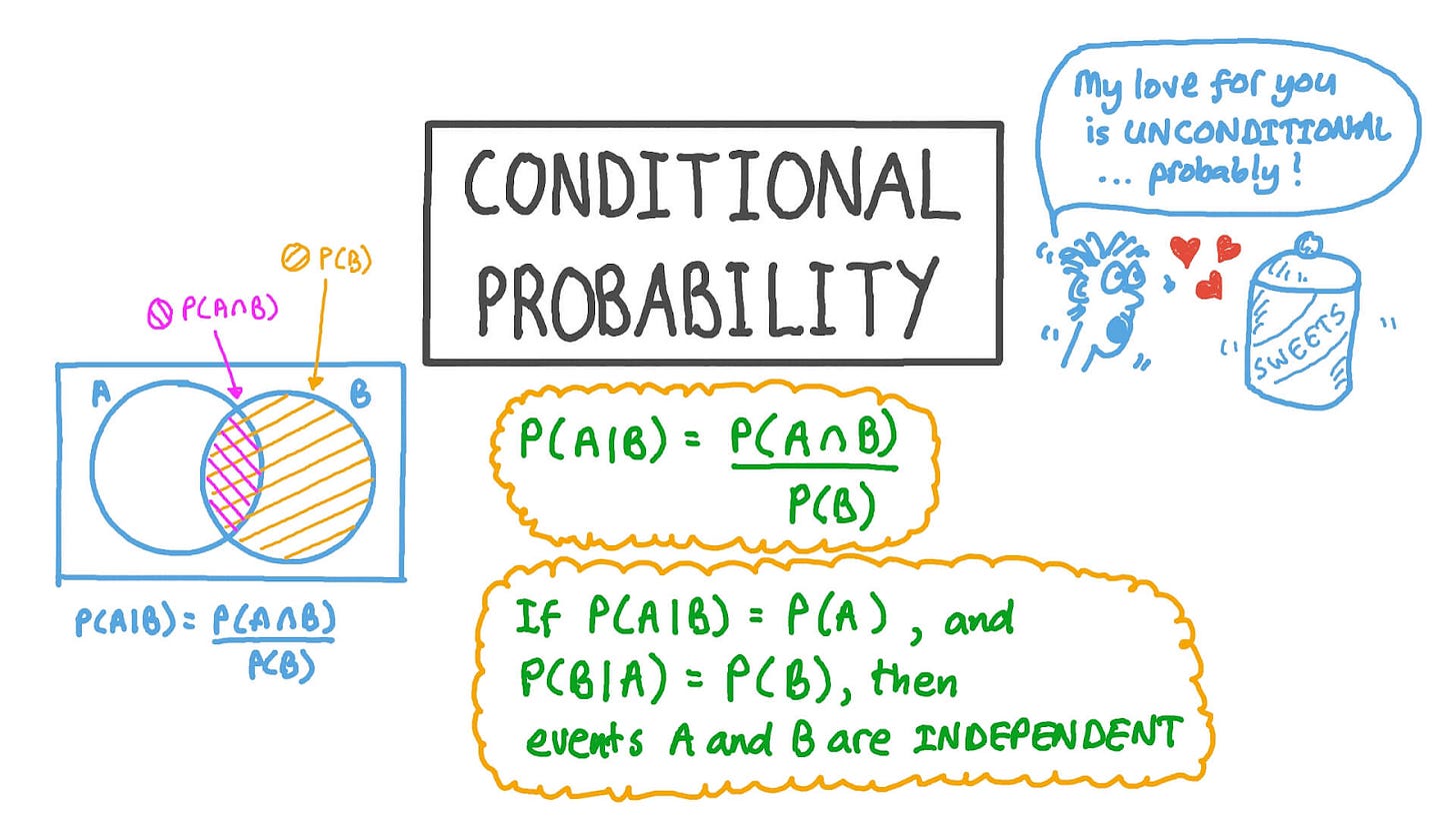
To restate the operation we calculated, either in our heads or with a computer: p(y|x) What is the conditional probability of y given x? Given x data (E), what is the probable output? Dog.
ChatGPT, similarly is essentially, given your input text, what is the likely output text? Starting with next word prediction, given “The,” what is the likely next word, similar to autofill on your iPhone.
Frequentist vs Bayesian Statistics
Probability is mostly broken into two camps. Frequentist methods focus on discrete sets of observed data and long-term frequencies, providing straightforward estimation and hypothesis testing techniques. On the other hand, Bayesian approaches consider previous assumptions and quantify uncertainty using posterior distributions. I think of this as “this is what I believed before and with this much room for error, after the new thing I just saw, this is now what I think generally and with this much error.”
Frequentist - Solely uses observable data. More simple and commonly used in simple systems. Discrete.
Bayesian - Incorporates prior knowledge, creates beliefs, and updates posterior distributions using observed data. Continuous.
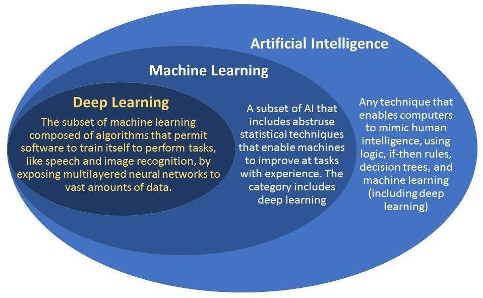
Artificial Intelligence, Machine Learning, and Deep Learning
Be wary when people use the term AI–it is annoyingly broad and includes simplistic linear functions that you learned in middle school. AI can include simple if-then statements. This technically fits the probabilistic definition we mentioned earlier, but it is just not that impressive.
Machine learning goes deeper but still in a simpler, hands-on way than deep learning that requires less data. While deep learning is an exciting field, the fundamentals of machine learning are necessary to understand its progress, and there are many instances where ML is a more effective tool than DL.
We should remember that deep learning is included within machine learning, albeit in a less structured way that relies on large amounts of data and generalized structure to self-learn. Deep learning has risen to prominence as society enters a regime of mass data and computation, where it has proven itself to exceed human levels of pattern recognition than even humans in chess, go, and now some parts of language.
Training, Supervised Learning, and Unsupervised Learning
When you are building any one of these models, you feed the model data. This data can be raw, or it can contain features. Raw data would be like feeding the model stock price data over time as a string of price values. A feature would be like taking price and dividing it by earnings, creating a price/earnings ratio, which may be a valuable, man-made data point for the model to learn
Supervised learning is when you train a model on both input and the output. This would be like if you fed images of a cat with the label of ‘cat’ and images of a dog with the label ‘dog’.
Unsupervised learning would be like if you fed cat and dog images with no labels and asked the computer to simply figure out the difference between the two. Unsupervised learning aims to find hidden patterns or intrinsic structures in data. While the use of unsupervised methods such as Principal Components Analysis (PCA) has advanced, the effectiveness of unsupervised learning has been disappointing to date.
2. Linear Algebra
The purpose of me writing this isn’t to go super deep into the math, rather to extract the intuition in a simple way. But some of the math will be necessary to go on. To set the stage, I will introduce an example. Say you are building a model that takes in 5 variables to predict an employee’s salary. The variables are all numeric and this is run by a linear regression model.
Years of Education
Years of Experience
Market Capitalization of the Company ($mm)
Hours worked per week
# of Subordinates
We log these variables as a vector in “feature space.” Feature space is a helpful way to visualize our features in “abstract vector space”. The vector x = [x1,x2,x3,x4,x5] where x inputs are represented as xi scalars.
If there were two variables, one can easily imagine plotting these points into a graph that looks something like this. You could also imagine graphing 3 variables in 3-dimensional “feature space.” This, however, is where our natural conception of space leaves us. What about 4 variables, 5, what about 1,000? What does that look like?
The best method I’ve heard to date is pioneered by leading researcher, Geoffrey Hinton. It goes as such: you look at a 3-dimensional graph and say 5 really loud!
Matrix Multiplication
There’s a lot here on matrix multiplication. I’m just dismayed that my 6th grade teacher was right and I did need to know this stuff after all. For the math to be clean, matrix multiplication requires conformable matrices.
Dot Product is important when we take two equal length vectors or matrices and combine them into a single value. This is a computationally inexpensive way of reducing matrices into a scalar.
Eigendecomposition [video] is a method used to decompose a matrix into a set of eigenvectors and eigenvalues. This is pretty hard for me to work with.
3. Probability and Information Theory
Probability theory is a mathematical framework for representing uncertain statements. Information theory is a branch of mathematics that revolves around quantifying how much information is present in a signal. The basic intuition behind information theory is that unlikely information is more valuable than likely information. (Information Theory of Startups - 2024)
Conditional Probability - a relatively simple concept that we discussed earlier. P(y|x).
Expectation, Variance, and Covariance
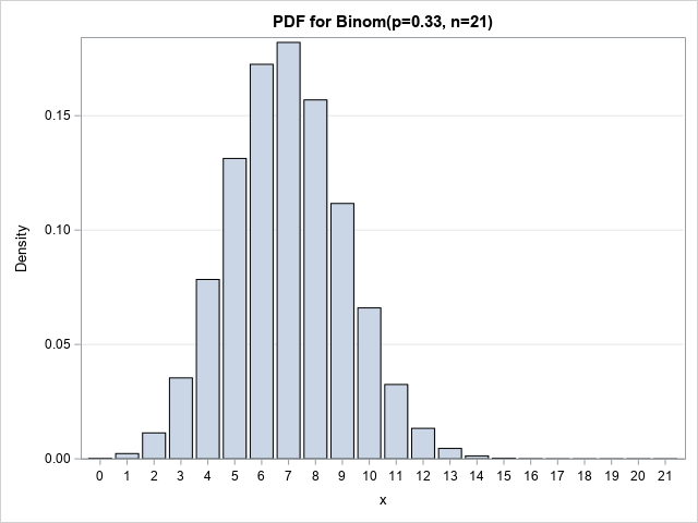
Another important concept is the “Expectation” denominated 𝔼. P in this sense is a complete distribution and p if it is a sample set. So we can calculate this in both a discrete, limited way and a continuous way.
This reads as: “The ‘expectation’ or expected value of x drawn from set P is the sum of f(x) times P(x) for all possible values of x.”
𝔼x~P [f(x)] =P(x)f(x)
Bayes’ Rule
Often, we find ourself in a situation where we need to know P(y|x) and need to know P(x|y). If we know P(x), we can compute this using Bayes’ Rule, which will also come in more handy later.
Bayesian Inference is a method of statistical inference in which Bayes' theorem is used to update the probability for a hypothesis as more evidence or information becomes available. This is learning in action. When you type words into ChatGPT, there is also an inference occurring. The model is learning from your input text and it is updating its context of the situation. Mechanics below:
Initialize the parameters θ with a prior belief.
For each data point or batch of data, compute the likelihood.
Update the posterior distribution using the likelihood and prior.
This process iteratively refines the parameter estimates.
Lastly, variance, covariance, and standard deviation are very important calculations in ML
Covariance gives a sense of how two values are related. In Project Delta ∆, we used a cov. matrix
Variance tells us how close our expected values are to the actual values.
Standard deviation is the sqrt of the variance
4. Numerical Computation
This is a relatively short chapter, which is good, because it highlights really just one super important concept.
Gradient-Based Optimization
Remember when we talked about E, T, and P? We are optimizing task T by maximizing performance P given experience E.
This is the most important concept of machine learning. Using the loss function, which is essentially all of the “expected values” compared to the “actual values” and the difference between the two representing error, we can optimize the function by minimizing the error. In other words, we are aiming to minimize the sum of each P(y|x).
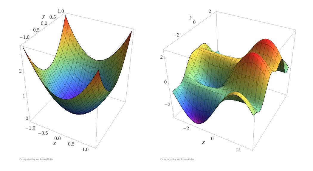
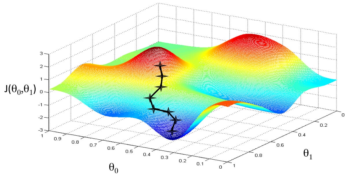
In linear, 2-dimensional convex space, this is super straightforward. You can optimize by finding the derivative = 0. In 3-dimensional space, it becomes more difficult but still simple with convex mapping. When there are multiple local minima, like in the picture on the right, it becomes more difficult.
Optimization is achieved by taking the derivative of the loss function, which gives us the slope of the function at that point. Now that we know the slope, we know the optimal step to descend the hill. Best case, we converge at the global minimum rather than falling into local minima (or saddle regions discussed later). Here, our variables have been optimized to the best fit equation.
Stochastic Gradient Descent
An extension of gradient descent, which is often considered slow and unreliable. This is the most used training methodology, often paired with momentum. Often, a small batch of samples (1-100) are drawn uniformly from the training set.
For large models, this is much quicker and does a reasonably good job. In many cases, the exact minimum is not needed. Local minima will often do just fine and so a computationally efficient way to drive reasonably good results is what is used.
5. Machine Learning Basics
In contrast to the above chapter, there is a ton of stuff in here. I am going to try to keep it simple. This was a great chapter that tied together all of the math we learned so far.
Basic types of learning algorithms:
Classification
Classification with Missing inputs
Regression
Transcription
Machine translation
Structured output
Anomaly detection
Synthesis and sampling
Imputation of missing values
Denoising
Density estimation and probability mass function estimation
The Training Process
The model is usually trained on a training set of the training data. This does not include the validation set data. ~80% is used for the training subset and learning the parameters and ~20% for the validation subset and estimating the generalization error. Though there are different strategies for this.
Hyperparameters
There are many indirectly important parameters, hyperparameters, that direct the learning process and control the algorithm’s behavior. These may be tuned through methods such as grid search or random search.
Strength of weight decay: λ
Capacity: degree of the polynomial
Learning rate
Model Layers
Epochs
Building a Machine Learning Algorithm
The recipe for building an algorithm is relatively simple in concept:
Use a specification of a dataset
Tie a cost function to performance relative to a task
Minimize a cost function using an optimization algorithm
Design decisions
Choosing the optimizer
Choosing the cost function
Choosing the form of the output units
Feedforward networks also introduce two new concepts
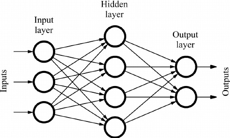
Hidden Layers
Activation Functions
Layers and units per layer.
First Layer: h(1) =g(1)(W(1)Tx+b(1))
h = hidden layer
g = activation function
W = weight matrix
x = input vector of the NN - the raw features fed into the input layer essentially
b = bias vector
Manifold Learning
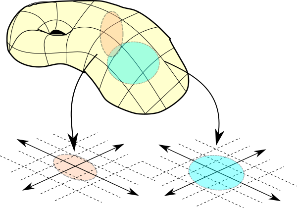
The manifold, as it ties to feature space and representation mapping, is probably my favorite concept in all of machine learning, yet also the most difficult to work with. The book outlines the manifold in the context of machine learning as “a connected set of points that can be approximated well by considering only a small number of degrees of freedom, or dimensions, embedded in a higher-dimensional space.
Put simply, you can imagine that multidimensional space, such as a 3-dimensional representation of the earth, has a 2-dimensional manifold like a giant piece of paper within. This is useful in the sense that we can take representations and reduce them into lower dimensional space, which may reasonably capture the concepts.
When I think of the manifold, I imagine computation space similar to how Stephen Wolfram defines Rulial Space and generative AI space [video]. You see there are sparse islands in what is regarded as massive interconcept space. Take for instance the below gradient of possible concepts of cat pictures. If you move far in a particular direction, you may charter into “dog” concept space, where the pictures begin looking like a cat-dog and eventually a dog.
For many reasons, this is probably one of the most important paradigms of AI. Interconcept space contains all possible concepts. Some not yet explored by human minds. One begins to imagine a world where a computer is left to iterate through interconcept space and explore various ideas, validating them, and becoming creative in its own way, innovating faster than any human could.
In Project Delta ∆, we also explore the potential to map ourselves, our identities, our writings, etc into interconcept space. By breaking down these concepts into detailed concepts and comparing them to others or other concepts, we can begin to define the fundamental nature of ourselves and benchmark it to society. The use cases here are endless.
The manifold hypothesis is that the probability distribution over images, text strings and sounds occurring in real life are extremely concentrated.
6. Deep Feedforward Networks
The model is provided with inputs in the form of variables and the model applies weights to the variables as optimized through a process called backpropagation, which is essentially just optimizing the gradient that we discussed prior.
As the inputs flow through the hidden layer(s), the model learns the relationships between them and the output on its own. This complex learning is the backbone of the advancements in modern AI. According to Goodfellow,
“Following the success of back-propagation, neural network research gained popularity and reached a peak in the early 1990s. Afterwards, other machine learning techniques became more popular until the modern deep learning renaissance that began in 2006.
Most of the improvement [between 1986 and 2015 can be attributed to larger datasets and computers].”
Non-Linearity
Machine learning creates a linear model that represents the underlying data. This is problematic as there are many functions that can not be represented in a purely linear way. These problems are solved through the introduction of activation functions (most prominently ReLU, rectified linear unit) that act similarly to human synapses and introduce non-linearity to enable the model to perform better. For small datasets, using rectifying non-linearities is more important than learning the weights of the hidden layers.
Non-linear models can no longer be solved in closed form but the advantages usually outweigh this fault and an iterative model for minimizing loss such as gradient descent is used.
7. Regularization for Deep Learning
A central problem in machine learning is creating models that not only perform well on the training data but also on new inputs. This requires generalization. Regularization offers up many methods in order to improve models ability to generalize on new data.
Some methods of regularization. Bold represents areas of interest for me.
L1 and L2 Parameter Regularization: parameter norm penalties that inhibit over-emphasis on various parameter weights.
Noise Robustness: purposefully introduce noise as an effective form of regularization
Dataset augmentation: introducing more data, even in synthetic form.
Early stopping: not allowing model to overfit
Parameter tying and parameter sharing
Bagging and Ensemble Methods: train models separately and average them
Dropout: computationally inexpensive way bagging by randomly pruning nodes and forcing generalization
Tangent Distance, Tangent Prop, and Manifold Tangent Classifier
Adversarial training: use the model to identify examples the model misclassified and works backwards to correct
Semi-supervised learning: tying a relationship between unlabeled and labeled data
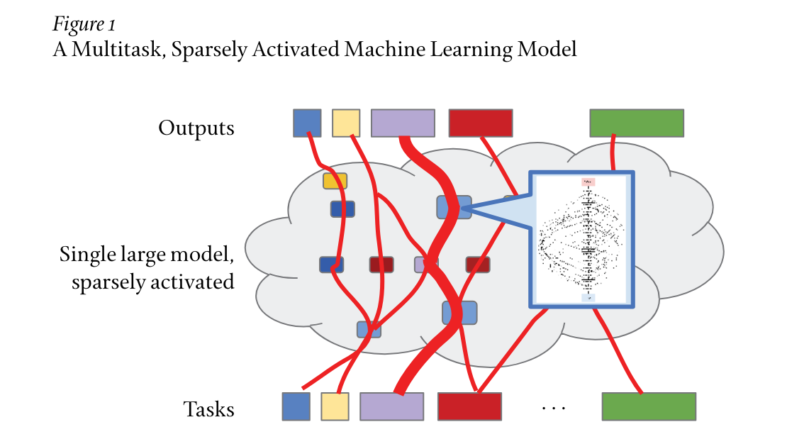
Multitask Learning: pooling examples from multiple learning tasks so that the models generalize. Multitask learning may hold significant breakthroughs for the field of deep learning.
Building a single machine learning system that can handle millions of tasks, and that can learn to successfully accomplish new tasks automatically, is a true grand challenge in the field of artificial intelligence and computer systems engineering.
8. Optimization for Training Deep Models
This doesn’t feel like a very useful introductory chapter for me right now other than the basic idea that when training a model, there are many ways to then optimize it.
Chapters and methods:
Empirical risk minimization
Surrogate loss functions and early stopping
Batch and minibatch algorithms
Plateus, saddle points, and other flat regions
Cliffs and exploding gradients
Long-term dependencies
Inexact gradients
Poor correspondence between local and global structure
Theoretical limits of optimization
Basic algorithms: SGD + momentum most notably
Parameter initialization strategies
Algorithms and adaptive learning rates: AdaGrad, RMSProp, Adam
Approximate second-order methods
Newton’s method
Conjugate gradients
BFGS
Continuation methods and curriculum learning
Some Interesting notes:
Nearly any deep model is essentially guaranteed to have a large number of local minima
In high-dimensional spaces, local minima are rare, and saddle points are more common
“It is more important to choose a model family that is easy to optimize than a powerful optimization algorithm”
Trends/Principles
There are some general trends we can identify as these technologies scale and become more useful. These trends are important to identify as we extrapolate use cases across industries and project out performance, which is often on an exponential ramp, into the future. There are also some paradoxes, unintuitive realizations, and unsolved mysteries that I will note.
I plan to add to this list over the years.
Principle 1: The Bitter Lesson
While not explicitly cited in the book, there are many parallel threads to Rich Sutton’s famous passage on The Bitter Lesson after 70 years of AI research.
“The biggest lesson that can be read from 70 years of AI research is that general methods that leverage
computation are ultimately the most effective, and by a large margin”
Humans are stubborn in thinking that there must be ways that our thinking is special. We aren’t special. Any hard-coded algorithms, special features, or attempts to mimic the human brain are steamrolled by large amounts of computation, data, and general methods in the long run. This is best seen in the success of DeepMind beating Kasparov in chess and the difficult-to-explain effectiveness of overparameterization. This brings me to principle 2.
Principle 2: The Big 3 - Talent, Data, and Computation
On a meta-note for the productivity of these models, if you want to build performant models, you can’t skimp on either of these three important resources. The confluence of these exponentially growing forces leads us into a future we cannot predict.
Talent: you need leading researchers, scientists, and engineers to build models that avoid pitfalls and maximize performance
Data: Machine learning is just sexy statistical modeling on top of data. If your data is corrupt, everything is broken. There is a nuance to this, that it seems massive amounts of data (scraping the internet) can outperform lesser amounts of clean data.
Compute: In order to run large scale models, large computation on a level orders of magnitude greater than you can imagine is needed.
Proxy for Talent: Research Papers - One strong indicator is the number of papers posted to the machine learning–related categories of arXiv, a popular paper preprint hosting service, with more than thirty-two times as many paper preprints posted in 2018 as in 2009 (a growth rate of more than double every two years).
[Would like to include a log graph of # of people in the space, computation dedicated towards it, and quantity of available data.]
Principle 3: Exponential Growth in Models
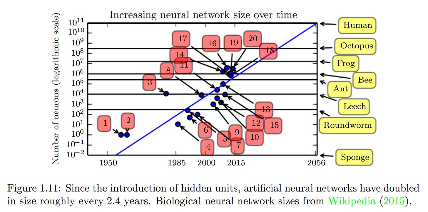
At the time of this book being published, artificial neural networks doubled in size roughly every 2.4 years.
This has since accelerated beyond Moore’s law.
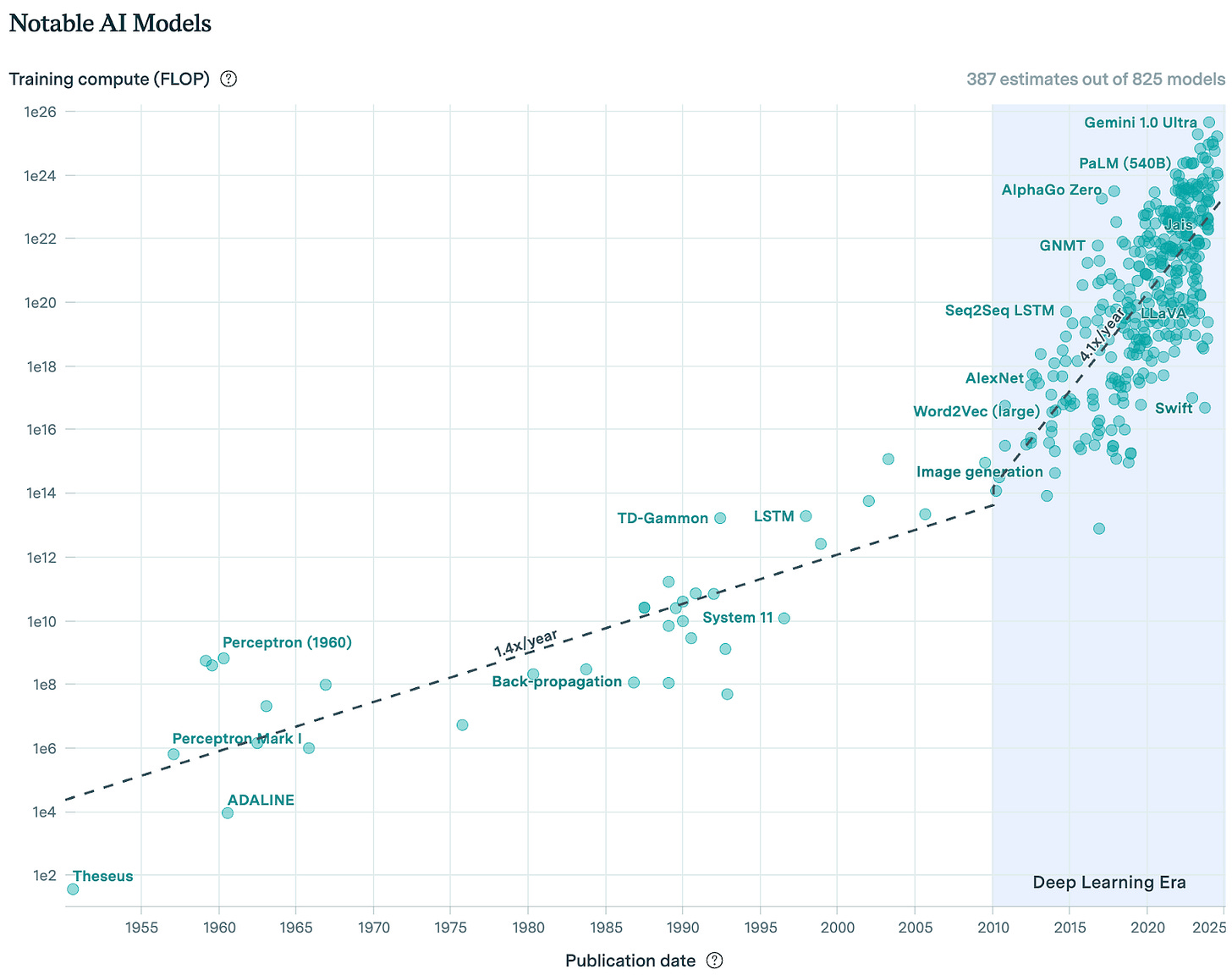
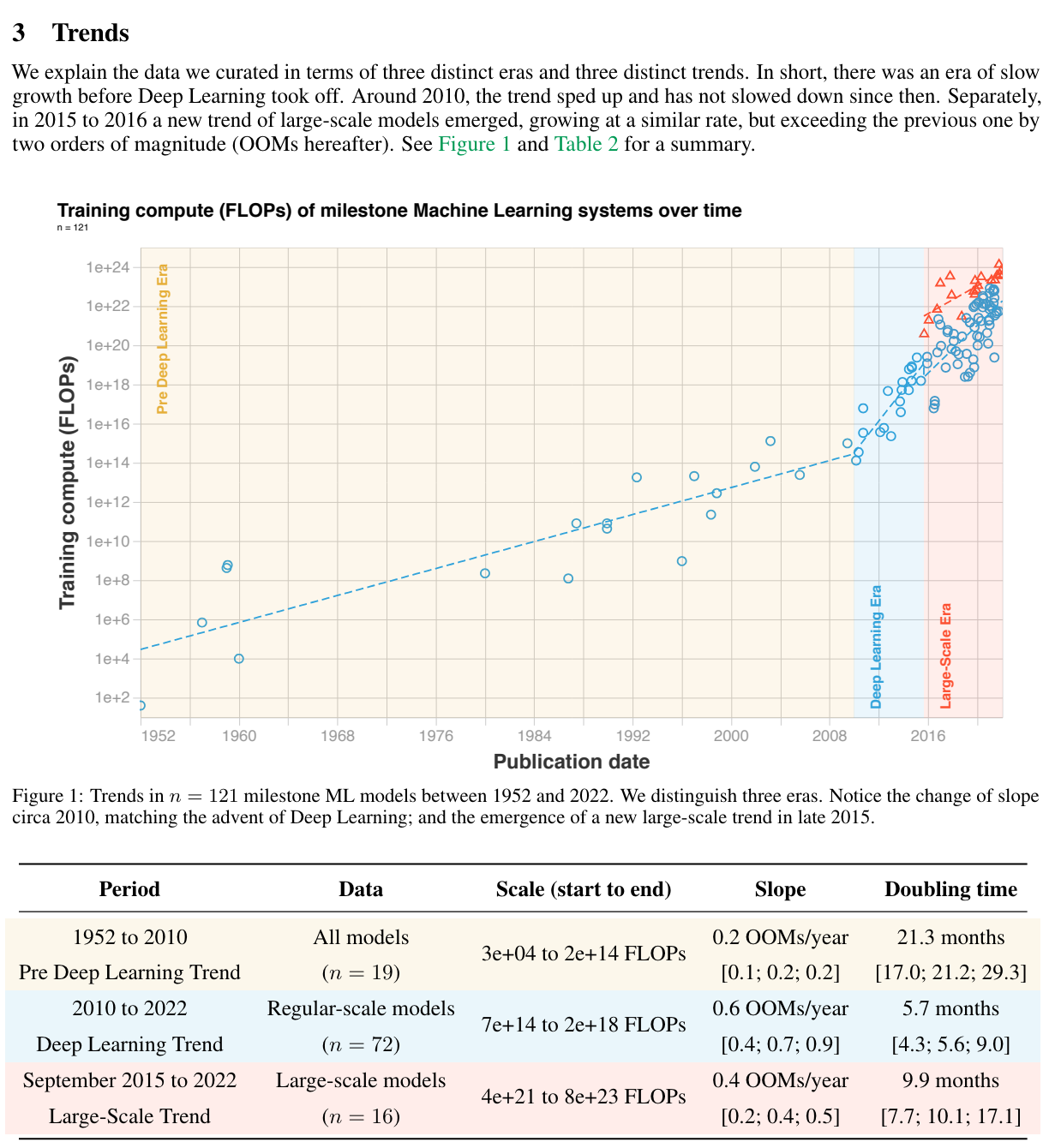
Since 2010, during the deep learning era we now find ourselves, the training compute used to create AI models has been growing at a rate of 4.1x per year. Most of this growth comes from increased spending, although improvements in hardware have also played a role.
Interactive Compute Graph and Parameter Graph.
If we assume this trend to continue forward, these models will have 1,342,265x more compute at scale in 10 years.
How does that change our world? Do we even have the infrastructure to sustain such a change?
A Golden Decade of Deep Learning: Computing Systems & Applications [Jeff Dean, Spring 2022]
“In 1990, we needed about one million times more computational power, not sixty-four times, for neural networks to start making impressive headway on challenging problems! Starting in about 2008, though, thanks to Moore’s law, we started to have computers this powerful
In 2004, we saw a nearly twenty-fold improvement for a neural network algorithm using a GPU. In 2008, computer scientist Rajat Raina and colleagues demonstrated speedups of as much as 72.6 times from using a GPU versus the best CPU-based implementation for some unsupervised learning algorithms.”
There are many variables that determine the growth of model power, and it is hard to pin down what the estimated growth in capability will be.
Principle 4: No Free Lunch Theorem
Theory stating that: averaged over all possible data-generating distributions, every classification algorithm has the same error rate when classifying previously unobserved points. Said differently, no machine learning algorithm is universally any better than any other.
Core Idea: NFLT states that no single algorithm performs best on all possible problems. Performance averages out across all possible tasks, meaning an algorithm that excels in one domain may perform poorly in another.
Principle 5: The Curse of Dimensionality
The "curse of dimensionality" refers to various phenomena that arise when analyzing and organizing data in high-dimensional spaces. These challenges become increasingly significant as the number of dimensions (features) grows. Here are the key aspects of the curse of dimensionality:
Increased Computational Complexity: As the number of dimensions increases, the computational cost for algorithms grows exponentially. This includes both the time required for computation and the amount of memory needed.
Sparsity of Data: In high-dimensional spaces, data points become exponentially far from each other, creating difficulty identifying meaningful patterns or clusters. Similarly, in high-dimensional spaces, the distances between points tend to become more uniform. Given different clusters of data are similarly spaced, it makes it difficult to distinguish between them.
Etc
Principle 6: Universal Approximation Theorem
In simple words, the universal approximation theorem says that neural networks can approximate any function. One can imagine that a computer can do anything, withstanding the possibility that we live in a computationally irreducible world, as Wolfram says.
“States that a feedforward network with a linear output layer and at least one hidden layer with any ‘squashing’ activation function (such as the logistic sigmoid) can approximate any Borel measurable function from one finite-dimensional space to another with any desired nonzero amount of error, provided that the network is given enough hidden units.”
APPENDIX
Computational Framework for the Brain
The most fascinating part of all the Machine Learning research I’ve done to date, starting with work at Quant, Nephra, CS 440 (Artificial Intelligence), and independent research, is that it’s provided me with a surprisingly useful framework to view the world. At times more useful than anything I’ve learned in psychology, the foundations of machine learning foundationally define learning and how the mind works that picks up where many qualitative models of psychology leave off.
The most humbling lesson of all is just how seemingly fast these models are taking off. The uniqueness of human intelligence is put into question. Computers are on track to exponentially outstrip our intelligence to make us the future equivalent of ants. We can debate when that day will come, but it’s no longer a question of if, and it seems increasingly likely that it will be in our lifetime.
In an always prescient 2007 glance into the future, Thiel describes an inevitable world of volatile risk, where technology bears the potential energy to wipe out everything we love. How does one prepare for such a future?
(Trimmed)
“But the world has not yet come to an end, and there is no easy telling how long the twilight of the modern age will endure. What then must be done, by the Christian statesman or stateswoman aspiring to be a wise steward for our time?
The negative answers are straightforward. There can be no return to the archaic world or even to the robust conception of the political envisioned by Carl Schmitt.
Unlike Strauss, the Christian statesman or stateswoman knows that the modern age will not be permanent, and ultimately will give way to something very different.
And so, in determining the correct mixture of violence and peace, the Christian statesman or stateswoman would be wise, in every close case, to side with peace. There is no formula to answer the critical question of what constitutes a “close case”; that must be decided in every specific instance. It may well be that the cumulative decisions made in all those close instances will determine the destiny of the postmodern world. For that world could differ from the modern world in a way that is much worse or much better—the limitless violence of runaway mimesis or the peace of the kingdom of God.”
Peter Thiel, The Straussian Moment
The Singularity, the Capitalist, and the Technologist
It is alarming that today can be viewed as the twilight of the modern age. How did we get here? And why doesn’t anyone seem to acknowledge this reality?
“The technological singularity is a hypothetical future point in time at which technological growth becomes uncontrollable and irreversible, resulting in unforeseeable consequences for human civilization.”
There is a movement, e/acc (effective accelerationism), that is terribly misguided in this sense. The optimistic case for tech is always that “humans find a way to contain it.” But there is a real sense in which that is impossible in this case. And where humans are either killed off entirely or forced to integrate. In which case, you stumble upon unanswerable questions of whether you’re still human at all?
Self-interested capitalists, and I’d argue now technologists, build the thing that will kill them.
“When it comes time to hang the capitalists, they will vie with each other for the rope contract.” - Lenin
“Why does Frankenstein create the Monster? Frankenstein believes that by creating the Monster, he can discover the secrets of “life and death,” create a “new species,” and learn how to “renew life.” He is motivated to attempt these things by ambition. He wants to achieve something great, even if it comes at great cost.”
Just as the capitalists vie for the rope contract, the naive technologists, out of pride, end the world they hoped to save.






Interesting principles!